5 Proteomic Landscapes of CCOC

root.dir <- rprojroot::find_rstudio_root_file()
knitr::opts_chunk$set(echo = TRUE)
knitr::opts_knit$set(root.dir = root.dir )
source(file.path(root.dir,'src/util.R'))
library(stringr)
library(dplyr)
library(plyr)
library(tidyr)
library(tibble)
library(ggplot2)
library(pheatmap)
library(heatmaply)
library(corrplot)
library(cowplot)
library(factoextra)
library(siggenes)
library(DT)

5.1 Loading and Transforming RPPA data

Reverse Phase Protein Arrays (RPPA) is processed by Functional Proteomics RPPA Core at MD Anderson Cancer Center. A total of 66 samples (2 replicates for each cell line + medium) were probed with 453 antibodies. rppa_ab_info.csv contains antibody infromation and rppa_normal.csv contains 453 log2-transformed normalized relative protein level for each samples.

ab.info.path <- 'data/RPPA/rppa_ab_info.csv'
ab.info.df <- read.csv(ab.info.path)
ab.info.df$Gene.Name <- lapply(ab.info.df$Gene.Name,function(x){str_replace_all(x,"\\[PAR Modification\\]","PAR")})
rppa.normal.path <- 'data/RPPA/rppa_normal.csv'
#taking out ab_info and NormalLog2 
rppa.normal.df <- read.csv(rppa.normal.path)
rppa.normal.df <- rppa.normal.df[,colSums(is.na(rppa.normal.df)) == 0]
ab.validation.status <- rppa.normal.df[4,-c(1:9)] %>% unlist %>% unname
rppa.normal.df <- rppa.normal.df[-c(1:8,10),]
names(rppa.normal.df) <- str_replace_all( rppa.normal.df[1,]," ","_" )
rppa.normal.df <- rppa.normal.df[-1,]
rppa.normal.df <- rppa.normal.df[!apply(is.na(rppa.normal.df) | rppa.normal.df == "", 1, all),]
rppa.normal.df <- rppa.normal.df[,colSums(rppa.normal.df != "") != 0 ]
cell.culture.type <- unname(sapply( rppa.normal.df["Sample_description"], function(x) str_extract(x,"(3D)|(2D)")))
cell.line <- sapply(rppa.normal.df$Sample_description, function(x){ y <- str_replace_all(x,"_[2-3]D_[1-2]$","")})
rppa.normal.df$Sample <- unname(sapply( rppa.normal.df["Sample_description"], function(x){ y <- str_replace_all(x,"_[1-2]$",""); str_replace_all(y,"-","_") }))
rppa.normal.df <- cbind( cell.line=cell.line, cell.culture.type=cell.culture.type , rppa.normal.df)
rppa.normal.df <- rppa.normal.df %>% filter(!str_detect(Sample_description,"NOSE16"))
#names(rppa.normal.df)<- c(names(rppa.normal.df)[c(1:9)], as.character(ab.name))
#names(rppa.normal.df)<- lapply(names(rppa.normal.df),function(x){str_replace_all(x,"\\[PAR Modification\\]","PARP")})
rownames(rppa.normal.df) <- str_replace_all(rownames(rppa.normal.df),"-","_")

5.2 Removing Samples from RPPA that failed QC

The following samples are excluded for further as they do not meet QC threshold set by MD Anderson RPPA core for having an overall low protein concentration:

• HCH1_3D_2

• JHOC9_3D_1

• JHOC9_3D_2

• OVTOKO_3D_1

rppa.normal.df <- rppa.normal.df %>% dplyr::filter(Sample != "JHOC9_3D") %>% dplyr::filter(Sample_description %notin% c("HCH1_3D_2","OVTOKO_3D_1"))

5.3 RPPA Experiment Summary

DT::datatable(ab.info.df %>% dplyr::count( Gene.Name,sort=TRUE),caption="Antibodies per gene count")

ab.phosphorylation.count <-sum(str_detect(ab.info.df$Antibody.Name,"_p"))
protein.count <- ab.info.df$Gene.Name %>% unlist %>% unique %>% length
ab.count <- ab.info.df$Gene.Name %>% unlist %>% length
str_glue("In this assay, **{ab.count}** probes were available to capture **{protein.count}** proteins in which **{ab.phosphorylation.count}** is phosphorylated")

In this assay, 453 probes were available to capture 392 proteins in which 91 is phosphorylated

5.4 Checking Technical Replicate Qulatity

5.4.1 Correlation plot

rppa.normal.df["Sample"] <- sapply( rppa.normal.df["Sample_description"], function(x){ y <- str_replace_all(x,"_[1-2]$",""); str_replace_all(y,"-","_") })


#calculating corrleation

M <- t(rppa.normal.df[,-c(1:10)] %>% dplyr::mutate_all(as.numeric))
colnames(M) <- rppa.normal.df$Sample_description
#colnames(M) <- sapply(colnames(M), function(x){ y <- str_replace_all(x," [0-9]$","")})
corrplot(cor(M,method = "spearman"),        # Correlation matrix
         method = "square", # Correlation plot method
         type = "full",    # Correlation plot style (also "upper" and "lower")
         diag = TRUE,      # If TRUE (default), adds the diagonal
         tl.col = "black", # Labels color
         bg = "white",     # Background color
         order = "hclust",
         #hclust.method= "centroid",
         hclust.method= "ward.D2",
         tl.cex = 0.6,
         col = NULL)       # Color palette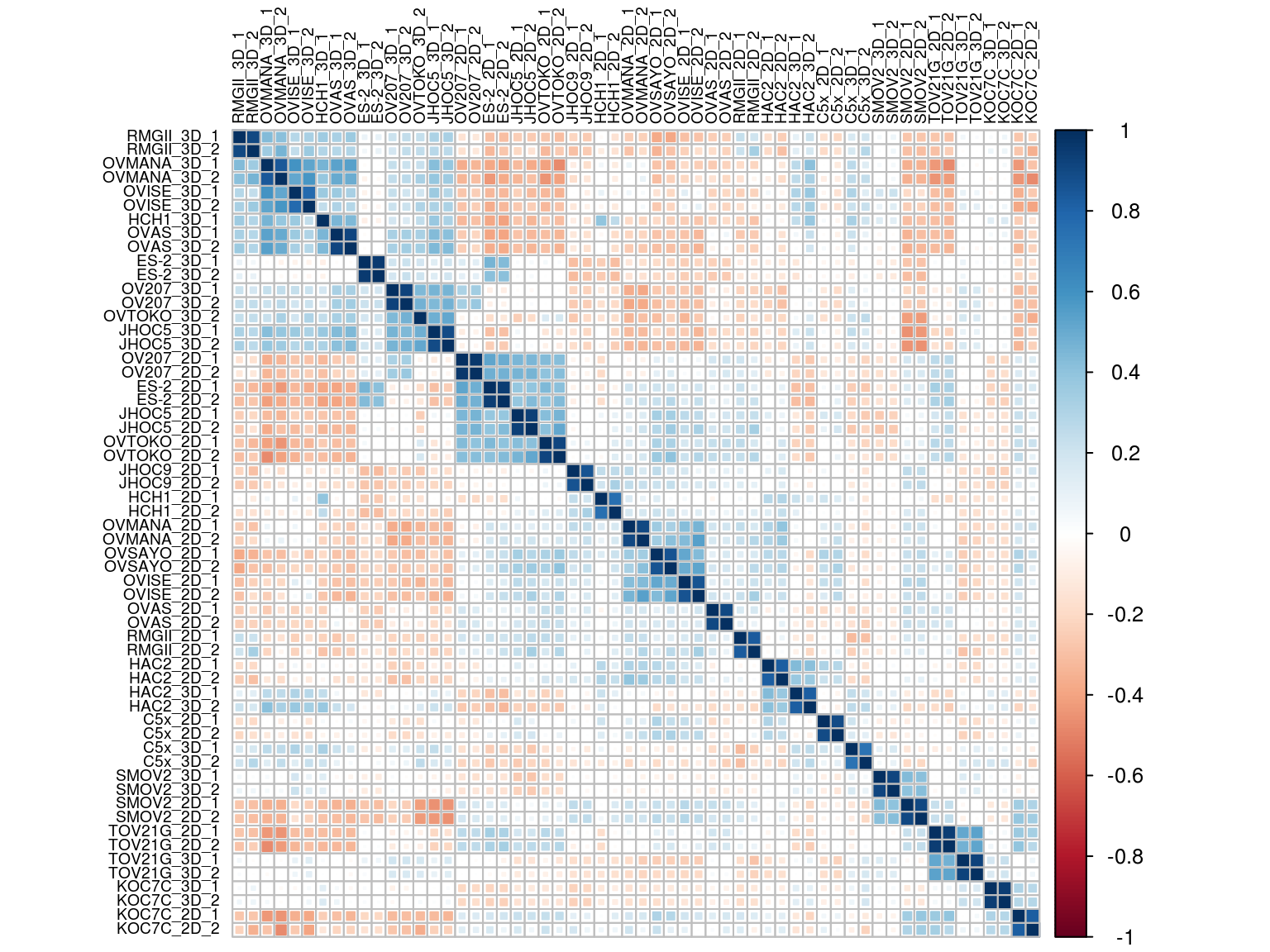

5.4.2 Scatter plot of protein level for each sample replicate

#get.pair <- function(x){ rppa.normal.df %>% filter(!! rlang::parse_expr(x)) %>% dplyr::select(Sample_description) }

#rppa.group <- sapply(unique(rppa.normal.df["Sample"]),function(x){ expr <- paste0('Sample == "', x , '"' ) ; get.pair(expr) })
rppa.group <- split(rppa.normal.df[,-c(1:5,7:10)] %>% dplyr::mutate_at(vars(-c("Sample")),as.numeric), f =rppa.normal.df$Sample)

rppa.group.plot <- lapply(rppa.group, function(df){ if(dim(df)[[1]] >1){
                                                    col.name <-rownames(df);
                                                    df <-data.frame(t(df)[-1,])%>% mutate_all(as.numeric)
                                                    ggplot(df,aes(x= .data[[ col.name[[1]] ]], y= .data[[ col.name[[2]] ]] ))+ geom_point() + theme_minimal()+geom_abline()}})

rppa.group.plot <- rppa.group.plot[lengths(rppa.group.plot) != 0]

plot_grid(plotlist = rppa.group.plot, align = "h")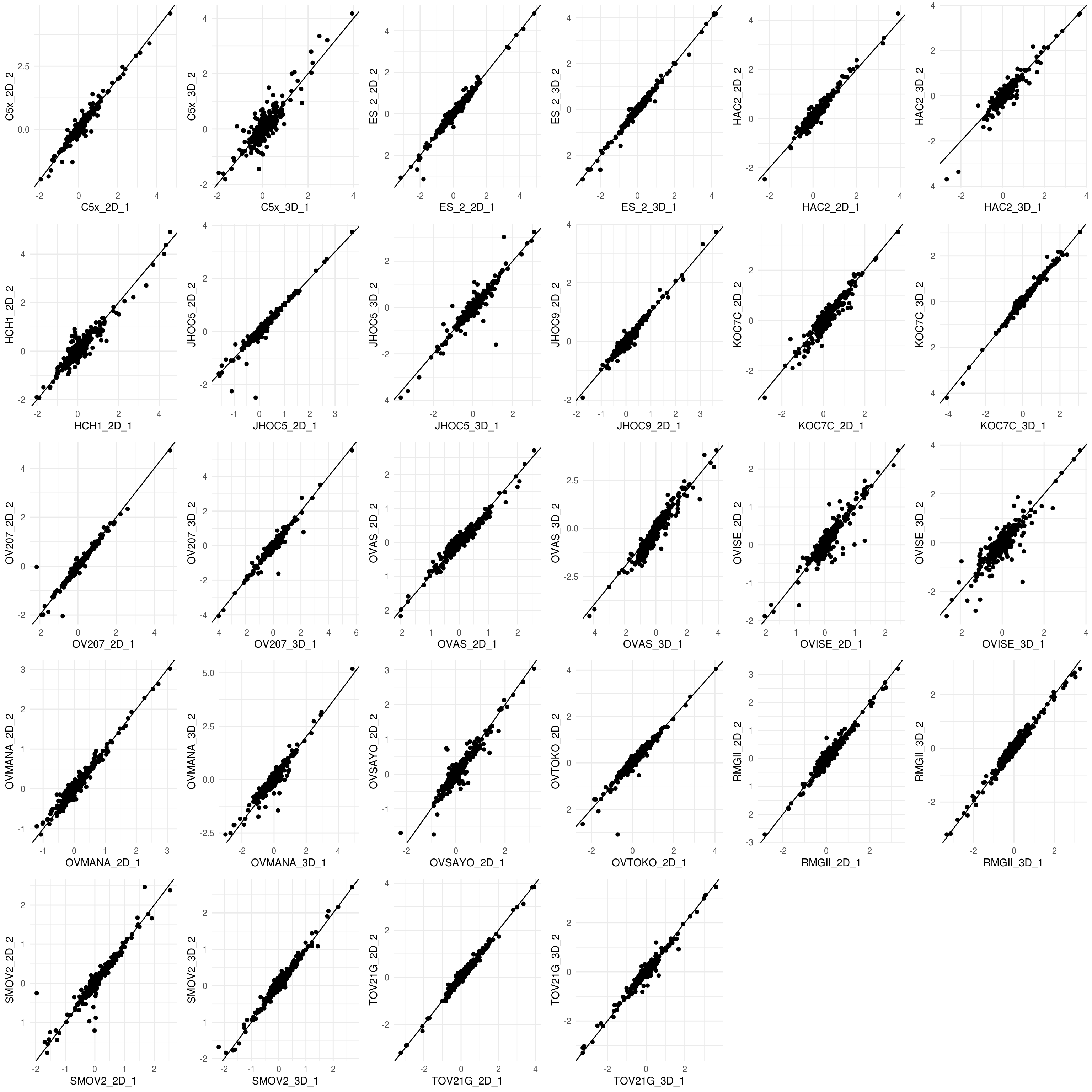

5.4.3 Heatmap for all sample replicates

heat.map.color <- viridis(n = 256, alpha = 1, begin = 0, end = 1, option = "viridis")
ann.colors <- list(cell.culture.type= c(`3D`= "#1B9E77",`2D` = "#D95F02"))

df <- as.data.frame(rppa.normal.df[c("cell.culture.type","cell.line")])
rownames(df) <- rppa.normal.df$Sample_description
select <- order( apply(M, 1, sd) ,
                decreasing=TRUE)
M <- apply(M,2,function(x){(x - mean(x)) / sd(x)})

pheatmap(M[select,] , cluster_rows=FALSE, show_rownames=FALSE, color=heat.map.color,
         cluster_cols=TRUE, annotation_col=df, fontsize = 8,annotation_colors=ann.colors, clustering_method= "ward.D2")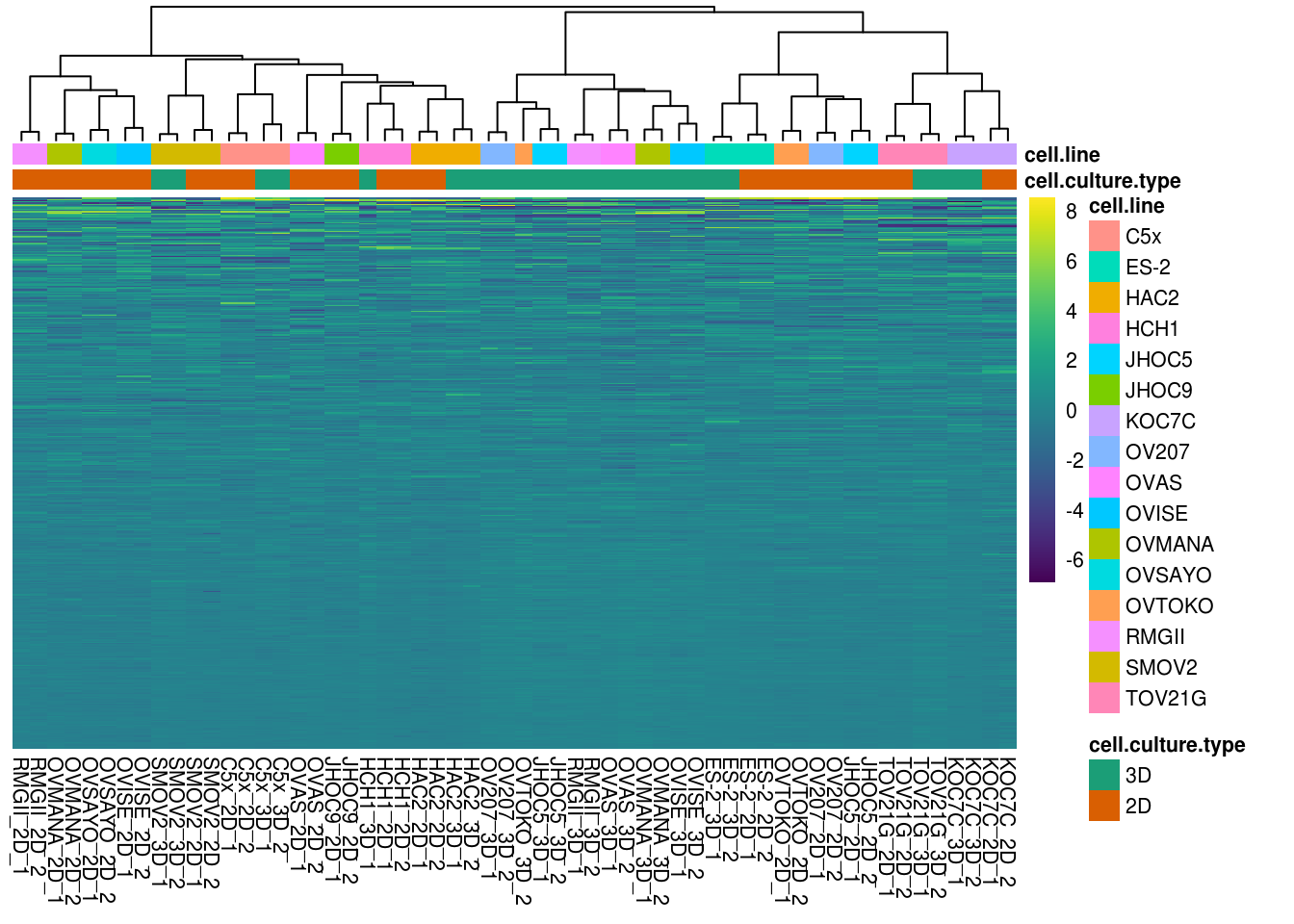

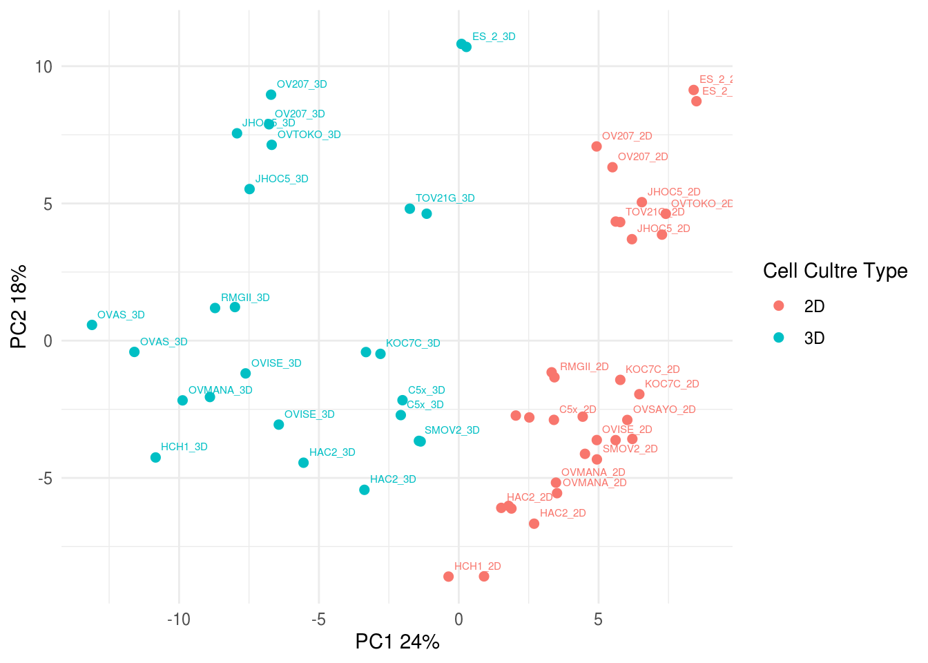
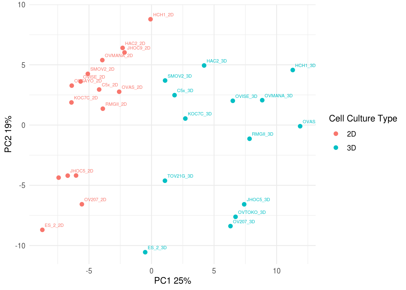
5.4.4 PCA plot all sample replicates

5.5 Merging replicates

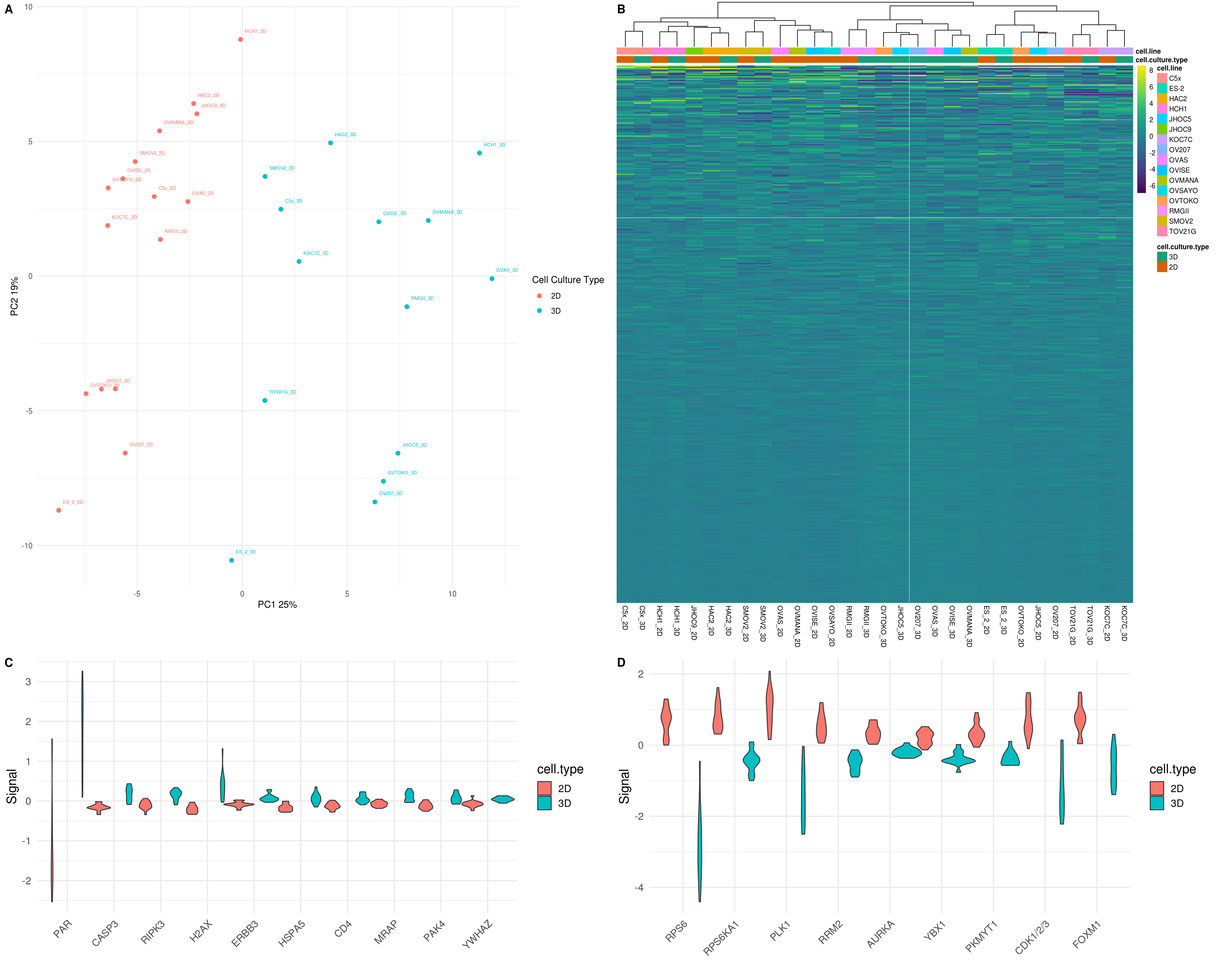
To conduct differenial protein expression analysis, replicates for each samples were merged by taking the mean of log2-transformed normalized relative protein level. PCA and Heatmap was carried out to confirm the merged samples were similar to individual replicates.

rppa.normal.df.combined <- rppa.normal.df[,-c(3:5,7:10)] %>% group_by(Sample,cell.culture.type,cell.line) %>%  mutate_at(vars(-c("Sample","cell.line","cell.culture.type")),as.numeric) %>% summarise_if(.,is.numeric,"mean")
rownames(rppa.normal.df.combined) <-rppa.normal.df.combined$Sample

## Warning: Setting row names on a tibble is deprecated.

5.5.1 Heatmap for merged RPPA data

M <- t(rppa.normal.df.combined %>% as.data.frame %>%dplyr::select(!c(Sample,cell.culture.type,cell.line)))
colnames(M) <- rppa.normal.df.combined$Sample
#geting metadata from rppa table
df <- as.data.frame(rppa.normal.df[c("cell.culture.type","cell.line")])
rownames(df) <- rppa.normal.df$Sample_description
df<- df %>% unique
rownames(df) <- sapply(rownames(df), function(x){ y <- str_replace_all(x,"_[1-2]$",""); z<- str_replace_all(y,"-","_") ; return(z)})
#rppa.normal.df.combined.heatmap <- merge(rppa.normal.df.combined, df, by.x="Sample", by.y="row.names")
select <- order( apply(M, 1, sd) ,
                decreasing=TRUE)
M <- apply(M,2,function(x){(x - mean(x)) / sd(x)})

heat.map<- pheatmap(M[select,] , cluster_rows=FALSE, show_rownames=FALSE,color=heat.map.color,
         cluster_cols=TRUE, annotation_col=df, fontsize = 8,annotation_colors=ann.colors, clustering_method= "ward.D2")

heat.map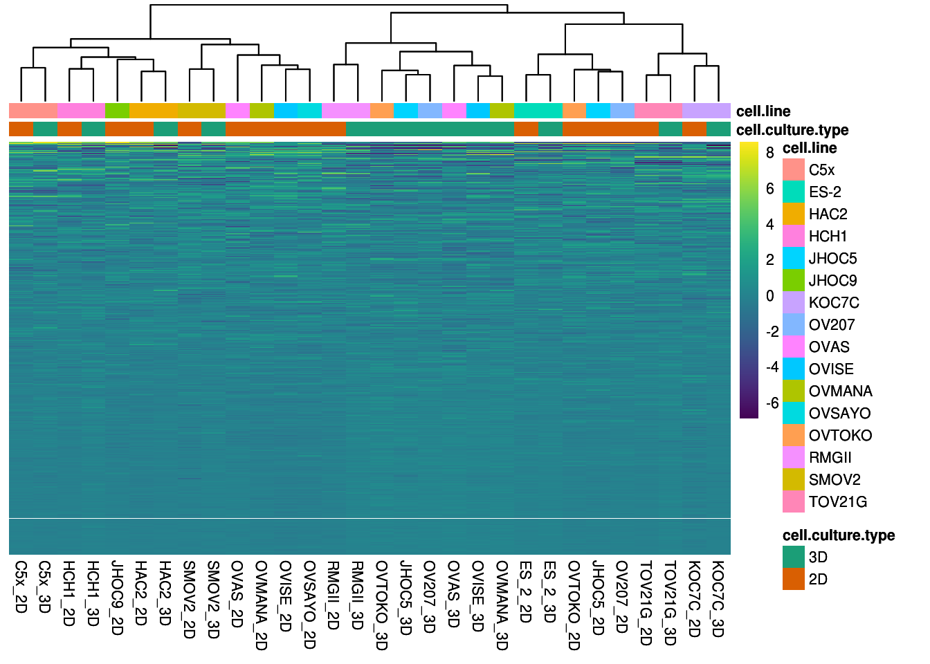

5.5.2 PCA for merged RPPA data

## Warning: Setting row names on a tibble is deprecated.

5.6 Significance Analysis of Microarray (SAM)

5.7 SAM Results

5.7.1 plot

sam.result <- sam( t(pca.tbl), sapply(rppa.normal.df.combined$cell.culture.type, function(x) { if (x == "2D") 0 else 1} ), method=d.stat,  gene.names = names(pca.tbl))


plot(sam.result) 

## To obtain a SAM plot, delta has to be specified in plot(object,delta,...).

5.7.2 table

knitr::kable(sam.result@mat.fdr)

Delta	p0	False	Called	FDR	cutlow	cutup	j2	j1
0.1	0.4159848	371.17	420	0.3676217	-0.2962185	0.1596744	199	232
1.1	0.4159848	32.23	214	0.0626504	-1.9398355	1.7717970	97	336
2.1	0.4159848	0.94	108	0.0036206	-3.4676973	3.1939353	45	390
3.2	0.4159848	0.01	45	0.0000924	-4.8968783	5.3570293	38	446
4.2	0.4159848	0.00	27	0.0000000	-5.9973094	7.3867023	26	452
5.2	0.4159848	0.00	18	0.0000000	-7.0261086	Inf	18	453
6.2	0.4159848	0.00	8	0.0000000	-8.3942860	Inf	8	453
7.2	0.4159848	0.00	5	0.0000000	-9.6834131	Inf	5	453
8.2	0.4159848	0.00	2	0.0000000	-11.9922925	Inf	2	453
9.3	0.4159848	0.00	0	0.0000000	-Inf	Inf	0	453

5.8 SAM Results for ∆ = 1.21

FDR threshold is set to be less than 5% which will make the value of parameter delta be somewhere between 1.009075 and 1.009076. Rounding it up to 1.21 for further analysis. NB The delta estimate method seems to be heuristic which might yield different delta in each runs that lead to different # of total DE protein. However, delta doesn’t affect top ranked DE proteins.

5.8.1 SAM plot

findDelta(sam.result, fdr = 0.05)

## The threshold seems to be at 
##      Delta Called      FDR
## 5 1.207411    208 0.050158
## 6 1.207412    207 0.048994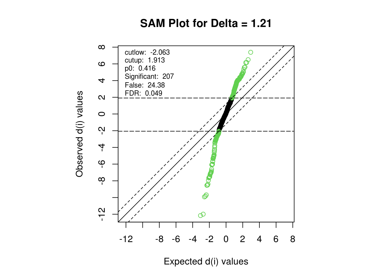

delta <-1.21
plot(sam.result,delta)

5.8.2 SAM summary

sam.genes<- summary(sam.result, delta)
knitr::kable(sam.genes@mat.fdr)

Delta	p0	False	Called	FDR	cutlow	cutup	j2	j1
1.21	0.4159848	24.38	207	0.0489938	-2.063406	1.913195	95	341

5.8.3 SAM protein table

gene.table <- sam.genes@mat.sig %>% mutate_if(is.numeric,round,4) %>% rownames_to_column("Antibody.Name.in.Heatmap") %>% mutate(gene.ab= factor(Antibody.Name.in.Heatmap,levels=ab.info.df$Antibody.Name.in.Heatmap, labels=ab.info.df$Gene.Name)) %>% left_join(ab.info.df[c("Antibody.Name.in.Heatmap","Validation.Status")],by="Antibody.Name.in.Heatmap") %>% dplyr::select(-c("Row"))
DT::datatable(gene.table,colnames = c("Ab","d.value","standard deviations","unadj p-val","q-val","Fold Change","Genes","validation status"),extensions =c('Buttons','Scroller'), options = list(
    dom = 'Bfrtip',
    buttons = c('copy', 'csv', 'excel', 'pdf', 'print'),
    "scrollX"= TRUE
  )) %>%
    formatStyle(
        'Antibody.Name.in.Heatmap',
        `font-size` = '12px',
    )

5.9 Top 10 SAM up/down-regulated proteins for ∆ = 1.21

5.9.1 Boxplot for top 10 SAM up/down-regulated proteins for ∆ = 1.21

#remapping pca_tbl with gene name
names(pca.tbl) <- factor(names(pca.tbl),levels=ab.info.df$Antibody.Name.in.Heatmap, labels=ab.info.df$Gene.Name)

## Warning: The `value` argument of `names<-` must be a character vector as of tibble 3.0.0.

n <- 10
up.gene.idx <- sam.genes@mat.sig[order(sam.genes@mat.sig$d.value, decreasing=TRUE),]$Row[1:n]
down.gene.idx <- sam.genes@mat.sig[order(sam.genes@mat.sig$d.value),]$Row[1:n]

tbl.up <-data.frame(cell.type=rppa.normal.df.combined$cell.culture.type, stack(pca.tbl[up.gene.idx]))
up.plot<- ggplot(tbl.up, aes(x=ind, y=values, fill=cell.type))+ geom_violin(width=1.3) + xlab("") + ylab("Signal")+scale_x_discrete(guide = guide_axis(angle = 45))+theme_minimal(base_size = 15) 

tbl.down <-data.frame(cell.type=rppa.normal.df.combined$cell.culture.type, stack(pca.tbl[down.gene.idx]))
down.plot <- ggplot(tbl.down, aes(x=ind, y=values, fill=cell.type))+ geom_violin(width=1.3) + xlab("") + ylab("Signal")+scale_x_discrete(guide = guide_axis(angle = 45))+ theme_minimal(base_size = 15)

plot_grid(plotlist = list(up.plot, down.plot))

## Warning: position_dodge requires non-overlapping x intervals

## Warning: position_dodge requires non-overlapping x intervals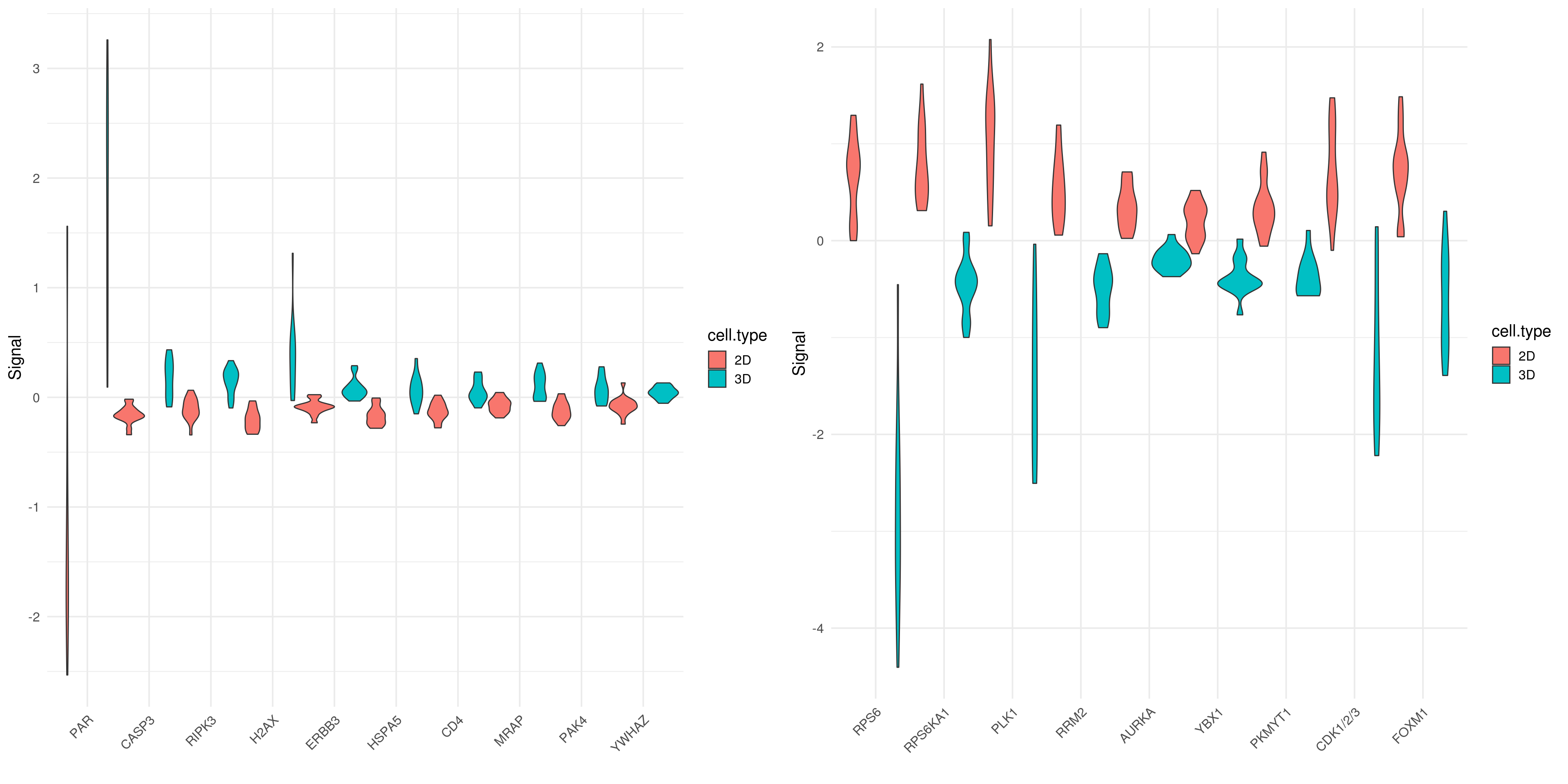

5.9.2 Heatmap for top 10 SAM up/down-regulated proteins for ∆ = 1.21

Subsetting the genes of ineterest from previous heatmap link text top 10 up-regulated protein doesn’t show too much varaince among each cell lines except PRAP (PAR-R-C). On the other hand,top 10 down-regulated proteins show strong differentiation

5.9.2.1 static heatmap

rownames(M) <- factor(rownames(M),levels=ab.info.df$Antibody.Name.in.Heatmap, labels=ab.info.df$Gene.Name)
up.heatmap <- pheatmap(M[up.gene.idx,] , cluster_rows=FALSE, color=heat.map.color ,
         cluster_cols=FALSE, annotation_col=df, fontsize = 8,annotation_colors=ann.colors, clustering_method= "ward.D2",main="Up")

down.heatmap <- pheatmap(M[down.gene.idx,] , cluster_rows=FALSE, color=heat.map.color,
         cluster_cols=FALSE, annotation_col=df, fontsize = 8,annotation_colors=ann.colors, clustering_method= "ward.D2", main="Down")

#plot_grid(plotlist = list(up.heatmap[[4]], down.heatmap[[4]]),labels=c("Up","Down"),align="hv")

5.9.2.2 Interactive heatmap

#top 10 SAM up-regulated protein
heatmaply(M[up.gene.idx,],  hclust_method = "ward.D2", main="Top 10 up-regulated proteins")

#top 10 SAM down-regulated protein
heatmaply(M[down.gene.idx,], hclust_method = "ward.D2", main="Top 10 down-regulated proteins")

## Warning in fix_not_all_unique(rownames(x)): Not all the values are unique - manually added prefix numbers

5.10 Figure 4. Targeted proteomic profiling of CCOC models

plot_grid(plotlist = list(pca.plot,heat.map[[4]],up.plot, down.plot), labels = "AUTO", ncol = 2, nrow=2,align ="hv", axis="tblr",rel_heights = c(2,1))

## Warning: position_dodge requires non-overlapping x intervals
## position_dodge requires non-overlapping x intervals

#plot_grid(plotlist = list(up.plot, down.plot))