3 Transcriptomatic Landscapes of CCOC models

3.1 Data Preparation and QC

root.dir <- rprojroot::find_rstudio_root_file()
knitr::opts_chunk$set(echo = TRUE)
knitr::opts_knit$set(root.dir = root.dir )
source(file.path(root.dir,'src/util.R'))
library(DESeq2)
library(dplyr)
library(tidyr)
library(tibble)
library(stringr)
library(knitr)
library(purrr)
library(itertools)
library(cowplot)
library(pheatmap)
library(heatmaply)
library(vsn)
library(ggplot2)
library(ggrepel)
library(gridExtra)
library(corrplot)
library(M3C)
library(UpSetR)
library(kableExtra)
library(biomaRt)

3.1.1 Loading gene expression data set

3.1.1.1 Loading count matrix

path.CCOC.RNA.count.table <- "data/RNA-seq/count_matrix/cell_line/KL-6799--04--27--2019_COUNTS.csv"
path.CCOC.RNA.count.table_2 <- "data/RNA-seq/count_matrix/cell_line/FA-9840--06--23--2020_COUNTS.csv"
tbls <- lapply(c(path.CCOC.RNA.count.table,path.CCOC.RNA.count.table_2),function(x){read.csv(file=x, row.names = 1,header = T, sep=",")} )

3.1.1.2 Loading Cell line

#import cell line name 
col.label.name.path <-'data/RNA-seq/CCOC_RNA_table_col.csv'
col.csv.tbl <- read.csv(file = col.label.name.path, header = T)

CCOC.RNA.count.table.col.name <- col.csv.tbl$KL.6799..04..27..2019_COUNTS %>% na_if("") %>% na.omit
CCOC.RNA.count.table_2.col.name <- col.csv.tbl$FA.9840..06..23..2020_COUNTS %>% na_if("") %>% na.omit
col.names <-list(CCOC.RNA.count.table.col.name,CCOC.RNA.count.table_2.col.name)
names(col.names)<- c(1,2)
tbls <- mapply(function(x,y){z<- paste(col.names[[y]],y);setNames(x,z) },tbls,names(col.names))

3.1.1.3 Making DGE object

3.1.1.3.1 merging tables into a single table

CCOC.RNA.count.table <- do.call(cbind,tbls)
CCOC.RNA.count.table <- CCOC.RNA.count.table %>% mutate_all(as.integer)

3.1.1.3.2 Making colData

#building colData
#cell.name <- as.factor(sapply(names(CCOC.RNA.count.table), function(x){ y <- str_replace_all(x,"-[1-2]$","")}))
cell.name <- as.factor(names(CCOC.RNA.count.table))
cell.batch <- as.factor(do.call(c,sapply(as.list(enumerate(tbls)),function(x){rep(x[[1]],length(x[[2]]))})))
cell.type <- as.factor(sapply(names(CCOC.RNA.count.table), function(x){if(str_detect(x,"3D")){"3D";}else "2D"}))
cell.line <- as.factor(cell.name %>% str_trim() %>% str_replace(., "[2-3]D-","") %>% str_replace(.,"-[0-9] [0-9]$",""))


colData <- data.frame(type=cell.type,name=cell.name , cell.line=cell.line, cell.batch= cell.batch)
rownames(colData) <- names(CCOC.RNA.count.table)
colData$name <- str_replace_all(colData$name,"-[0-9] [0-9]$","") %>% as.factor

3.1.1.3.3 making DESeq objecct

dds <- DESeqDataSetFromMatrix(countData = as.matrix(CCOC.RNA.count.table),
                                colData = colData,
                                design = ~ type +  cell.line + cell.batch )

dds <- estimateSizeFactors(dds)

bm <- get.bm()
protein.gene <- bm %>% dplyr::filter(gene_biotype == "protein_coding") %>% dplyr::filter( ensembl_gene_id %in% str_replace(rownames(dds),"\\..*$",""))

3.1.2 Checking Technical Replicate Qulatity

  ntd <- normTransform(dds)
  vsd <- vst(dds, blind=FALSE)

  msd.ntd <- meanSdPlot(assay(ntd), plot = F)
  msd.vsd <- meanSdPlot(assay(vsd), plot = F)
  # msd.rld <- meanSdPlot(assay(rld), plot = F)
  ymax <- max(c(max(msd.ntd$gg$data$py),
                max(msd.vsd$gg$data$py)))#,
                #max(msd.rld$gg$data$py)))
  p <- list()
  p[[1]] <- msd.ntd$gg + ggtitle('log2(n + 1)') + ylim(c(0,ymax))
  p[[2]] <- msd.vsd$gg + ggtitle('Variance stabilizing transformation') + ylim(c(0,ymax))
  # p[[3]] <- msd.rld$gg + ggtitle('Regularized log transformation') + ylim(c(0,ymax))
  library(cowplot)
  plot_grid(plotlist = p, align = 'hv', ncol = 2)#3)

## Warning: Removed 9 rows containing missing values (geom_hex).

## Warning: Removed 12 rows containing missing values (geom_hex).

3.1.2.1 Correlation plot

M <- counts(dds)
colnames(M) <- sapply(colnames(M), function(x){ y <- str_replace_all(x," [0-9]$","")})
corrplot(cor(M),        # Correlation matrix
         method = "square", # Correlation plot method
         type = "full",    # Correlation plot style (also "upper" and "lower")
         diag = TRUE,      # If TRUE (default), adds the diagonal
         tl.col = "black", # Labels color
         bg = "white",     # Background color
         order = "hclust",
         hclust.method= "ward.D2",
         tl.cex = 0.8,
         col = NULL)       # Color palette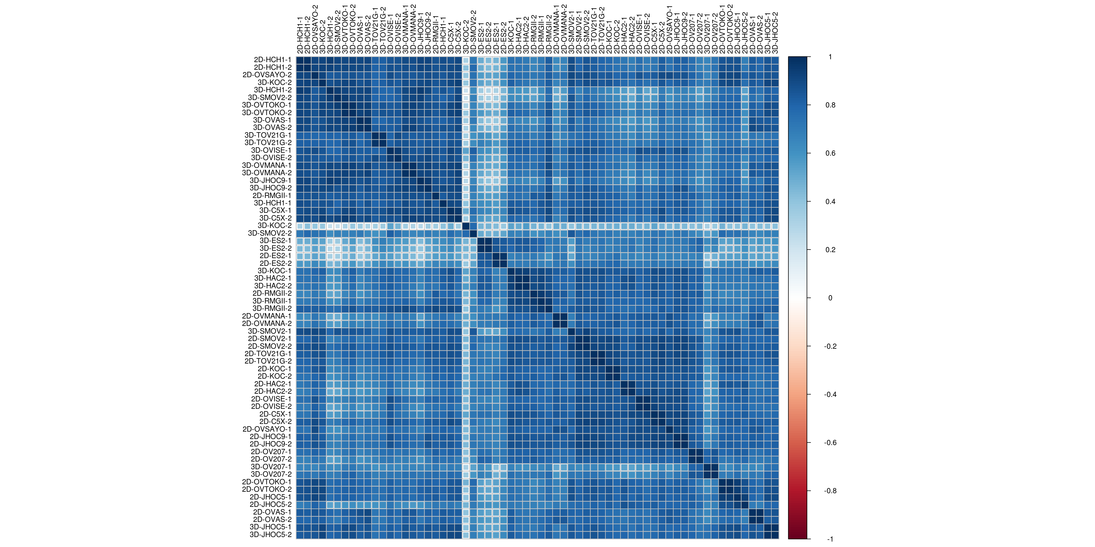

3.1.2.2 Sample to Sample Distance

  sampleDists <- dist(t(assay(vsd)))
  sampleDistMatrix <- sampleDists %>% as.matrix %>% as.data.frame
  rownames(sampleDistMatrix) <- rownames(colData(vsd))
  colnames(sampleDistMatrix) <- vsd$name
  colors <- heat.map.color <- viridis(n = 256, alpha = 1, begin = 0, end = 1, option = "mako")
  pheatmap(sampleDistMatrix, 
           clustering_distance_rows=sampleDists,
           clustering_distance_cols=sampleDists,
           clustering_method = 'ward.D2',
           col=colors, fontsize = 10, fontsize_row = 4)

3.1.2.3 PCA

  show.labels <- TRUE # change to TRUE if you want to show the sample IDs
  pcaData <- plotPCA.DESeqTransform(vsd, intgroup='type', returnData=TRUE)
  percentVar <- round(100 * attr(pcaData, "percentVar"))
  # adding cell line name into pcaData dataframe
  pcaData <- merge(pcaData, unique(colData[c("name","cell.line")]) , by="name")
  
  if(show.labels){
    #label <- pcaData$cell.name
    label <- pcaData$name
  }else{
    label <- NA
  }

PC.list <-c(1:4)
 g.plot <- lapply( PC.list , function(i){
  x=paste("PC",i,sep="")
  y=paste("PC",i+1,sep="")
  return( ggplot(pcaData[c(x,y,"cell.line","type")], aes( .data[[x]],  .data[[y]], color= cell.line ,shape=type ,label = label)) +
    geom_point(size=2) +
    xlab(paste0(x,": ",percentVar[i],"% variance")) +
    ylab(paste0(y,": ",percentVar[i+1],"% variance")) + 
    geom_text_repel(show.legend = F,size=1)+
    guides(colour="none"))+
    theme_minimal()
 })
 
plot_grid(plotlist = g.plot, align = "h")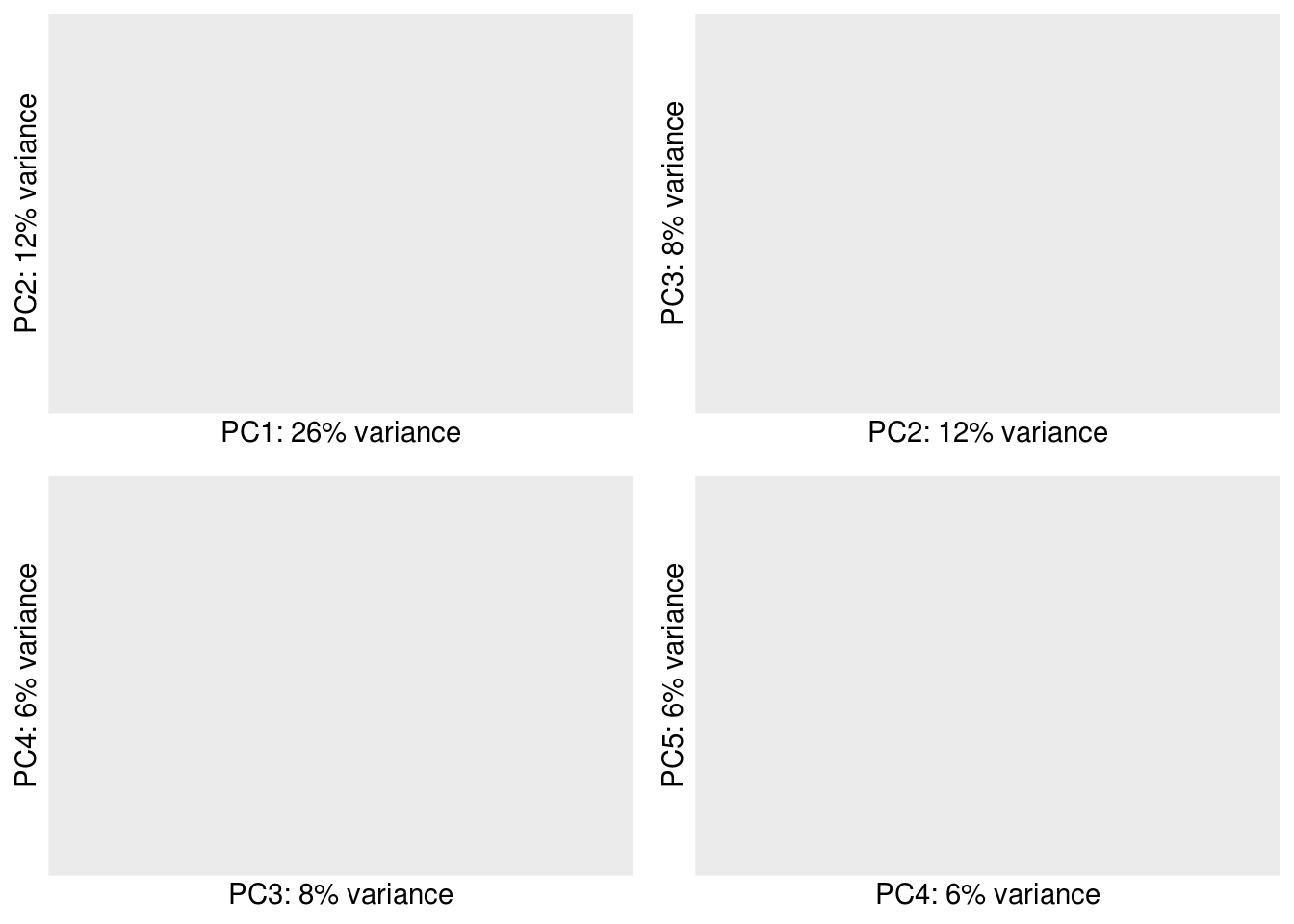

3.1.3 Merging Replicate and Data Prep for Downstream Anakysis

dds_c <- collapseReplicates(dds, dds$name)
ntd <- normTransform(dds_c)
vsd <- vst(dds_c, blind=FALSE)

  msd.ntd <- meanSdPlot(assay(ntd), plot = F)
  msd.vsd <- meanSdPlot(assay(vsd), plot = F)
  # msd.rld <- meanSdPlot(assay(rld), plot = F)
  ymax <- max(c(max(msd.ntd$gg$data$py),
                max(msd.vsd$gg$data$py)))#,
                #max(msd.rld$gg$data$py)))
  p <- list()
  p[[1]] <- msd.ntd$gg + ggtitle('log2(n + 1)') + ylim(c(0,ymax))
  p[[2]] <- msd.vsd$gg + ggtitle('Variance stabilizing transformation') + ylim(c(0,ymax))
  # p[[3]] <- msd.rld$gg + ggtitle('Regularized log transformation') + ylim(c(0,ymax))
  library(cowplot)
  plot_grid(plotlist = p, align = 'hv', ncol = 2)#3)

## Warning: Removed 8 rows containing missing values (geom_hex).

## Warning: Removed 11 rows containing missing values (geom_hex).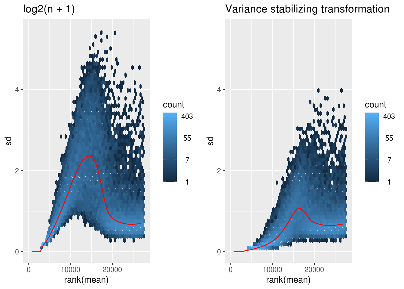

3.1.3.1 Correlation plot for Merged Data

M <- counts(dds_c)
colnames(M) <- sapply(colnames(M), function(x){ y <- str_replace_all(x," [0-9]$","")})
corrplot(cor(M),        # Correlation matrix
         method = "square", # Correlation plot method
         type = "full",    # Correlation plot style (also "upper" and "lower")
         diag = TRUE,      # If TRUE (default), adds the diagonal
         tl.col = "black", # Labels color
         bg = "white",     # Background color
         order = "hclust",
         hclust.method= "ward.D2",
         tl.cex = 0.8,
         col = NULL)       # Color palette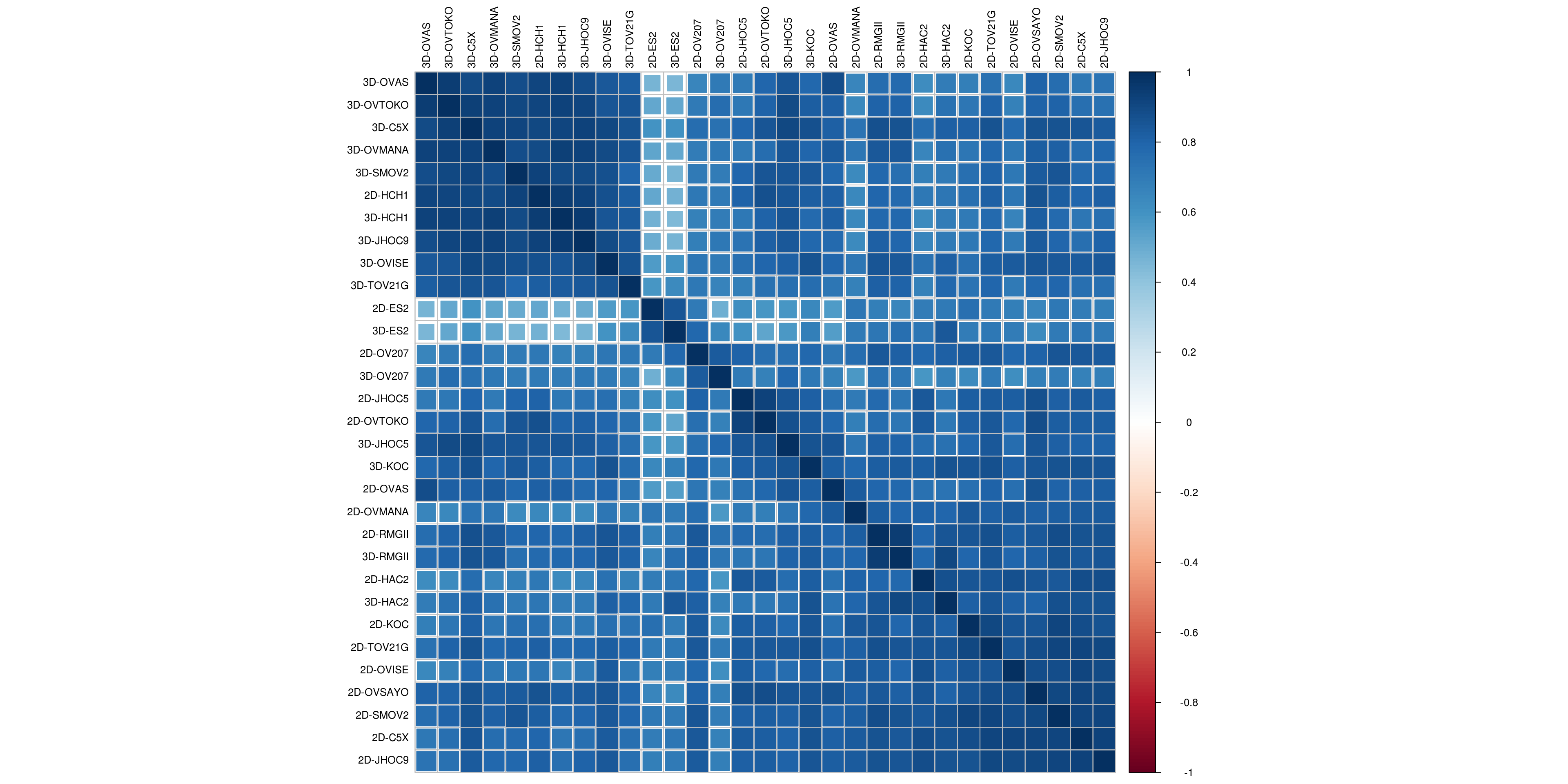

3.1.3.2 Sample to Sample Distance for Merged Data

  sampleDists <- dist(t(assay(vsd)))
  sampleDistMatrix <- sampleDists %>% as.matrix %>% as.data.frame
  rownames(sampleDistMatrix) <- vsd$name
  colnames(sampleDistMatrix) <- vsd$name
  colors <- heat.map.color <- viridis(n = 256, alpha = 1, begin = 0, end = 1, option = "mako")
  pheatmap(sampleDistMatrix, 
           clustering_distance_rows=sampleDists,
           clustering_distance_cols=sampleDists,
           clustering_method = 'ward.D2',
           col=colors, fontsize = 8, fontsize_row = 4)

3.1.3.3 PCA for Merged Data

  show.labels <- TRUE # change to TRUE if you want to show the sample IDs
  pcaData <- plotPCA.DESeqTransform(vsd, intgroup='type', returnData=TRUE)
  percentVar <- round(100 * attr(pcaData, "percentVar"))
  # adding cell line name into pcaData dataframe
  pcaData <- merge(pcaData, unique(dds_c@colData[c("name","cell.line")]) , by="name") %>% as.data.frame 
  
  if(show.labels){
    #label <- pcaData$cell.name
    label <- pcaData$name
  }else{
    label <- NA
  }

PC.list <-c(1:4)
 g.plot <- lapply( PC.list , function(i){
  x=paste("PC",i,sep="")
  y=paste("PC",i+1,sep="")
  return( ggplot(pcaData[c(x,y,"cell.line","type")], aes( .data[[x]],  .data[[y]], color= cell.line ,shape=type ,label = label)) +
    geom_point(size=2) +
    xlab(paste0(x,": ",percentVar[i],"% variance")) +
    ylab(paste0(y,": ",percentVar[i+1],"% variance")) + 
    geom_text_repel(show.legend = F,size=2)+
    guides(colour="none"))+
    theme_minimal()
 })
 
plot_grid(plotlist = g.plot, align = "h")

## Warning: ggrepel: 4 unlabeled data points (too many overlaps). Consider increasing max.overlaps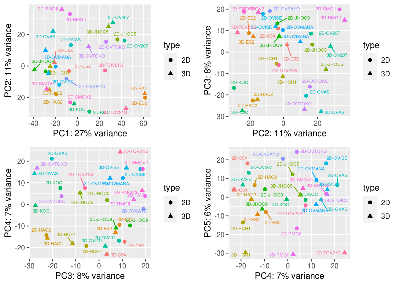

3.2 2D Consensus clustering

3.2.1 Data Preparation

df <- as.data.frame(colData(dds_c)[,c("cell.line","type")]) %>% filter(type =="2D")%>%mutate(rowname= rownames(.))
df <- merge(df, CCOC_mutation_table[,c(1,3:12)] %>%  dplyr::select(where(~ any(. != 0))), by.x="cell.line", by.y="cell_line", all.x=TRUE)
df <- merge(df, CCOC.Gly, by.x="cell.line", by.y="cell_line", all.x=TRUE ) %>% magrittr::set_rownames(.$rowname) %>% dplyr::select(-rowname)%>% dplyr::mutate( across(where(is.numeric), ~coalesce(., 0)))
ann_colors <- list(type= c(`3D`= "#1B9E77",`2D` = "#D95F02"))
vsd.gene.2D <- assay(vsd) %>% as.data.frame %>% dplyr::select(., starts_with("2D-")) %>% as.matrix
heat.map.color <- viridis(n = 256, alpha = 1, begin = 0, end = 1, option = "viridis")
#getting meta dataframe for 2D data
df <- get.2D.pheatmap.df()

col.list <- c(50, 500, 1000, 5000)
dds_c.mtx.select <- counts(dds_c,normalized=TRUE) %>% as.data.frame %>% dplyr::select(., starts_with(c("2D-","CCOC_"))) %>% as.matrix

pmap.df.list <- lapply(col.list, function(i){
  str_glue("#### Top **{i}** SD Gene ")
  select <- order(rowSds(dds_c.mtx.select),decreasing=TRUE)[1:i]
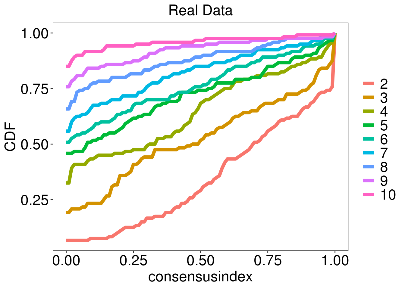
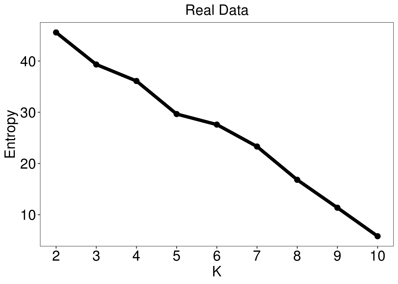
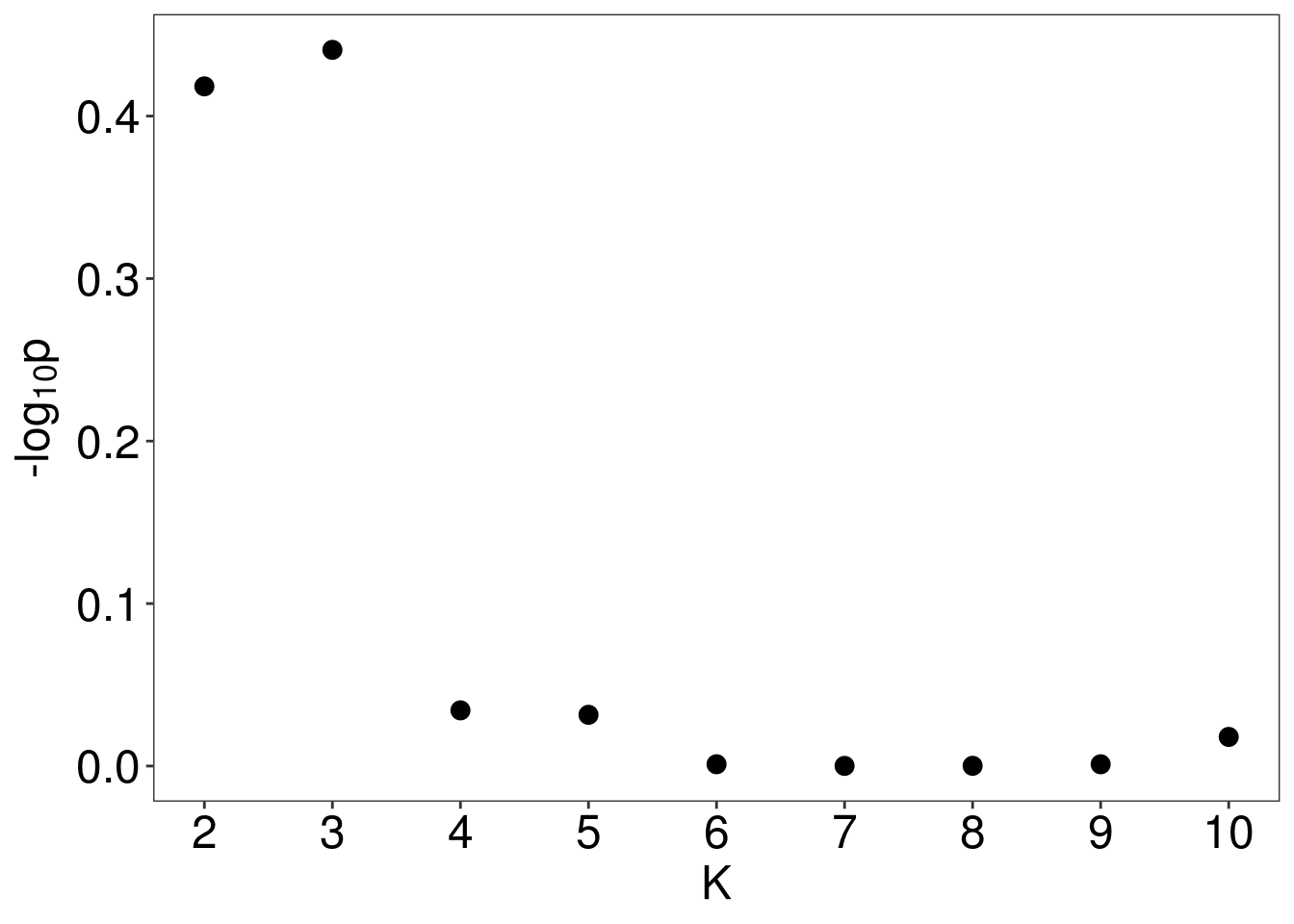
  test <- M3C(data.frame(vsd.gene.2D[select,]))
  k <- test$scores %>% mutate_all(as.numeric) %>% slice(which.max(RCSI)) %>% dplyr::select(K) %>% as.numeric
  cluster <- test$realdataresults[[k]]$ordered_annotation
  c.name <- factor( rownames(cluster) , labels=colnames(dds_c.mtx.select),levels=colnames(data.frame(vsd.gene.2D[select,])))
  rownames(cluster) <- c.name
  df <- merge(df,cluster, by.y="row.names" , by.x="row.names") %>% arrange(consensuscluster) 
  rownames(df)<- df$Row.names
  heat.map.ann.color <- viridis(n = k, alpha = 1, begin = 0, end = 1, option = "viridis")
  heat.map.ann.color.map <- unique(df$consensuscluster)
  heat.map.ann.color<- setNames(heat.map.ann.color.map,heat.map.ann.color.map)
  annotation_colors = list(consensuscluster=heat.map.ann.color)
  pmap <- pheatmap(vsd.gene.2D[select,], cluster_rows=TRUE, treeheight_row = 0, show_rownames=FALSE,
         cluster_cols=TRUE,color=heat.map.color , annotation_col=df, annotation_colors =annotation_colors ,fontsize = 8, annotation_legend = FALSE ,cutree_cols=k,clustering_method ="ward.D2")[[4]]
  return(structure(pmap,cluster=cluster))
  })

3.2.2 Expression of PI3CKA, ARID1A, HNF1B for consensus clustering of Top 5000 variable gene

cluster.assignment <- attr(pmap.df.list[[4]],"cluster")
cluster.expression.volin.df <- vsd.gene.2D %>% as.data.frame %>% dplyr::filter(str_detect(row.names(vsd.gene.2D),"PIK3CA|PIK3R1|ARID1A|HNF1B")) %>% rownames_to_column() %>% mutate(rowname=str_replace(rowname,"^.+_","")) %>% reshape2::melt() %>% merge(.,cluster.assignment,by.x="variable",by.y=0)

## Using rowname as id variables

xlabs <- paste(unique(cluster.expression.volin.df$consensuscluster),"\n(N=",table(cluster.expression.volin.df$consensuscluster)/length(unique(cluster.expression.volin.df$rowname)),")",sep="")
ggplot(cluster.expression.volin.df, aes(x=consensuscluster, y=value)) +geom_boxplot(aes(fill = rowname),width=0.5,position = position_dodge(0.8))+ geom_dotplot(aes(fill = rowname),binaxis = "y", stackdir='center', dotsize = 0.8,position = position_dodge(0.8))+ scale_x_discrete(labels=xlabs)+labs(y="Gene Epression Level (vsd)") + theme_classic()

## Bin width defaults to 1/30 of the range of the data. Pick better value with `binwidth`.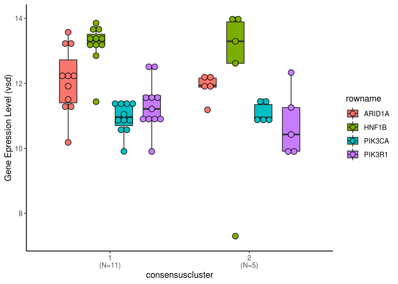

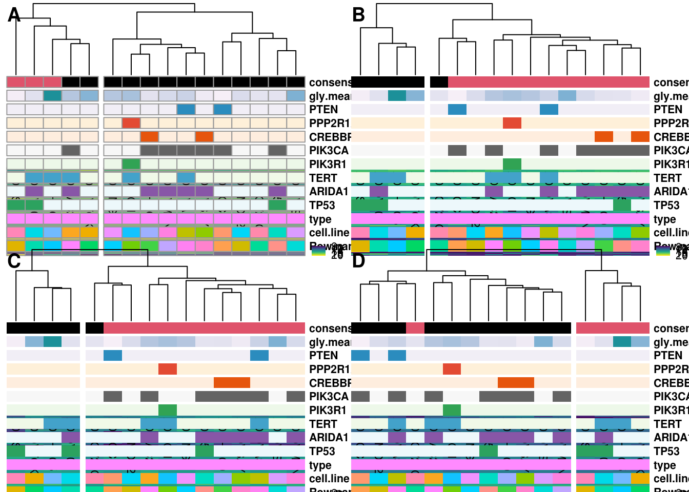
3.2.3 Global Heatmap for Consensus Clustering of Top 50, 500, 1000, 5000 variable genes

plot_grid( plotlist = pmap.df.list, ncol=2, nrow=2, labels="AUTO")

3.2.4 2D Consensus clustering DGE

dds.2D <- dds[,colData(dds)$type == "2D"]
colData(dds.2D) <- merge(colData(dds.2D),attributes(pmap.df.list[[4]])$cluster, by.x="name", by.y=0)
dds_c.2D.df <- merge(colData(dds_c),attributes(pmap.df.list[[4]])$cluster, by.x="name", by.y=0) %>% as.data.frame 
dds_c.2D.df <- merge(dds_c.2D.df,CCOC_mutation_table[,c(1,3:12)],by.x="cell.line", by.y="cell_line",all.x=TRUE) 
dds_c.2D.df <- dds_c.2D.df %>% mutate(PIK3=PIK3R1+PIK3CA+PTEN) %>% dplyr::select(-c(PIK3R1,PIK3CA,PTEN))
dds_c.2D.df <-  merge(dds_c.2D.df,CCOC.Gly,by.x="cell.line", by.y="cell_line",all.x=TRUE)%>% column_to_rownames("name")

design(dds.2D) <- ~ cell.batch + consensuscluster
dds.2D <- estimateSizeFactors(dds.2D)
dds.2D <- DESeq(dds.2D)

alpha <- 0.01
# get FC and pvalues (equivalent methods)
res.2D <- results(dds.2D, name="consensuscluster_2_vs_1", alpha = alpha)
resLFC.2D <- lfcShrink(dds.2D, coef = 3, type="apeglm")
resNorm.2D <- lfcShrink(dds.2D, coef = 3, type="normal")
resAsh.2D <- lfcShrink(dds.2D, coef = 3, type="ashr")
par(mfrow=c(1,4), mar=c(4,4,2,1))
yMax <- max(abs(c(res.2D$log2FoldChange, resLFC.2D$log2FoldChange, resNorm.2D$log2FoldChange, resAsh.2D$log2FoldChange)), na.rm = TRUE)
xMax <- max(c(plotMA(object = res.2D, returnData = T)[,1], plotMA(object = resLFC.2D, returnData = T)[,1], plotMA(object = resNorm.2D, returnData = T)[,1], plotMA(object = resAsh.2D, returnData = T)[,1]))
xlim <- c(1,xMax); ylim <- c(-yMax, yMax)
plotMA(res.2D, xlim=xlim, ylim=ylim, main="none", alpha = alpha) # default alpha = 0.10
plotMA(resLFC.2D, xlim=xlim, ylim=ylim, main="apeglm", alpha = alpha) # default alpha = 0.10
plotMA(resNorm.2D, xlim=xlim, ylim=ylim, main="normal", alpha = alpha) # default alpha = 0.10
plotMA(resAsh.2D, xlim=xlim, ylim=ylim, main="ashr", alpha = alpha) # default alpha = 0.10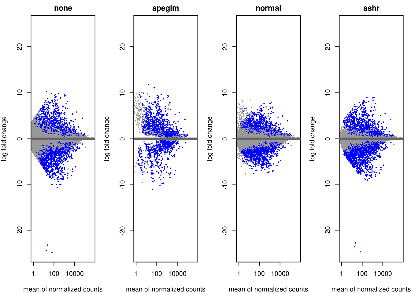

lsf.volcano <- lapply( list(res.2D,resLFC.2D,resNorm.2D,resAsh.2D), function(x){ 
  ggplot(data=data.frame(x) %>% na.omit %>% filter(abs(log2FoldChange) < 15), aes(x=log2FoldChange, y=-log10(padj))) +
        geom_point() + 
        theme_minimal() +
        geom_vline(xintercept=c(-0.6, 0.6), col="red") +
        geom_hline(yintercept=-log10(alpha), col="red") +
        xlim(-15,15) +
        ylim(-5,60)
        })

#do.call("grid.arrange", c(lsf.volcano, ncol=2, nrow=2))

do.call("plot_grid",c(lsf.volcano, labels ="auto"))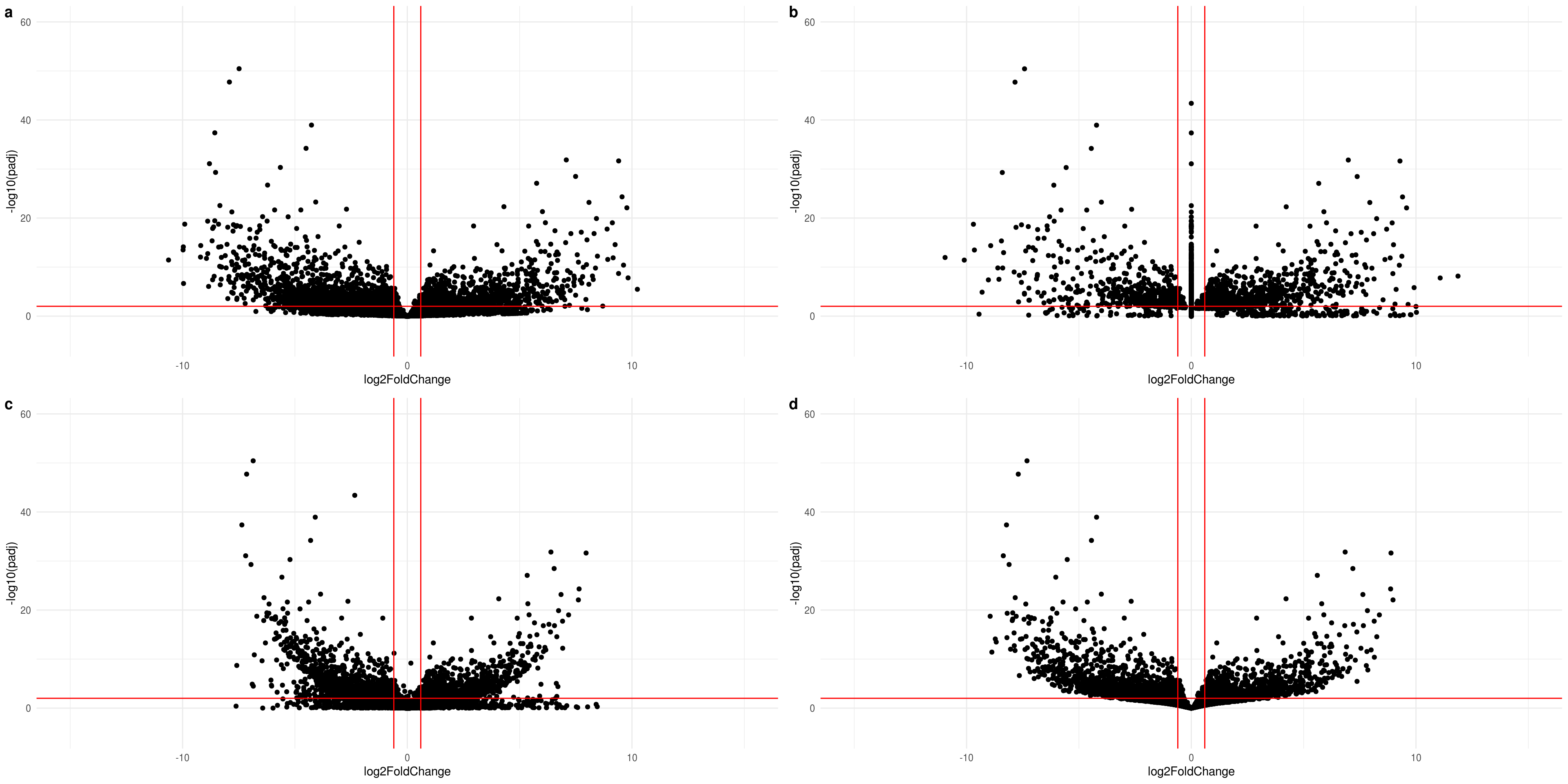

resAsh.2D <- resAsh.2D[resAsh.2D$padj < alpha & !(is.na(resAsh.2D$padj)),]
resOrdered <- resAsh.2D %>% as.data.frame %>% rownames_to_column %>% arrange(padj, desc(abs(resAsh.2D$log2FoldChange)))
resOrdered.up <- resOrdered %>% filter(resAsh.2D$log2FoldChange > 0)
resOrdered.down <- resOrdered %>% filter(resAsh.2D$log2FoldChange < 0)

#p.value.max <- max(resOrdered$padj[1:50])
#FC.min <- max(resOrdered$log2FoldChange[1:50])
#p.value.max <- max(resOrdered.down$padj[1:50])
#select <- which( (abs(df.resAsh$log2FoldChange < 0) & df.resAsh$padj <= p.value.max & !(is.na(df.resAsh$padj))) )

select <- which(rownames(vsd.gene.2D) %in% resOrdered$rowname & str_replace(rownames(vsd.gene.2D),"\\..*$","") %in% protein.gene$ensembl_gene_id  ) 
pheatmap(vsd.gene.2D[select,], cluster_rows=TRUE, show_rownames=FALSE,color=heat.map.color,
         cluster_cols=TRUE, annotation_col=dds_c.2D.df["consensuscluster"],fontsize = 7,clustering_method ="ward.D2")

3.2.4.1 Top 50 Genes Heatmap

select <- select[1:50]
heatmap.df<- dds_c.2D.df %>% dplyr::select(-c(type,sizeFactor,type,cell.line,cell.batch))
rownames(vsd.gene.2D) <- str_replace(rownames(vsd.gene.2D),"^.+_","")
pheatmap(vsd.gene.2D[select,order(heatmap.df$consensuscluster)], cluster_rows=TRUE,color=heat.map.color,
         cluster_cols=FALSE, treeheight_row=0, annotation_col=heatmap.df,fontsize = 7,clustering_method ="ward.D2")

3.2.4.2 DE genes list

 resAsh.2D <-data.frame(resAsh.2D) %>% mutate_if(is.numeric,round,4)
 DT::datatable(resAsh.2D,extensions =c('Buttons','Scroller'), options = list(
    dom = 'Bfrtip',
    buttons = c('copy', 'csv', 'excel', 'pdf', 'print'),
    "scrollX"= TRUE
  )) 

3.3 Differential gene expression

3.3.1 Cell meduim - 3D vs 2D

  dds <- DESeq(dds)

## using pre-existing size factors

## estimating dispersions

## gene-wise dispersion estimates

## mean-dispersion relationship

## final dispersion estimates

## fitting model and testing

## 5 rows did not converge in beta, labelled in mcols(object)$betaConv. Use larger maxit argument with nbinomWaldTest

3.3.1.1 Log fold change shrinkage

alpha <- 0.01
# get FC and pvalues (equivalent methods)
res <- results(dds, name="type_3D_vs_2D", alpha = alpha)
resLFC <- lfcShrink(dds, coef = 2, type="apeglm")
resNorm <- lfcShrink(dds, coef = 2, type="normal")
resAsh <- lfcShrink(dds, coef = 2, type="ashr")
par(mfrow=c(1,4), mar=c(4,4,2,1))
yMax <- max(abs(c(res$log2FoldChange, resLFC$log2FoldChange, resNorm$log2FoldChange, resAsh$log2FoldChange)), na.rm = TRUE)
xMax <- max(c(plotMA(object = res, returnData = T)[,1], plotMA(object = resLFC, returnData = T)[,1], plotMA(object = resNorm, returnData = T)[,1], plotMA(object = resAsh, returnData = T)[,1]))
xlim <- c(1,xMax); ylim <- c(-yMax, yMax)
plotMA(res, xlim=xlim, ylim=ylim, main="none", alpha = alpha) # default alpha = 0.10
plotMA(resLFC, xlim=xlim, ylim=ylim, main="apeglm", alpha = alpha) # default alpha = 0.10
plotMA(resNorm, xlim=xlim, ylim=ylim, main="normal", alpha = alpha) # default alpha = 0.10
plotMA(resAsh, xlim=xlim, ylim=ylim, main="ashr", alpha = alpha) # default alpha = 0.10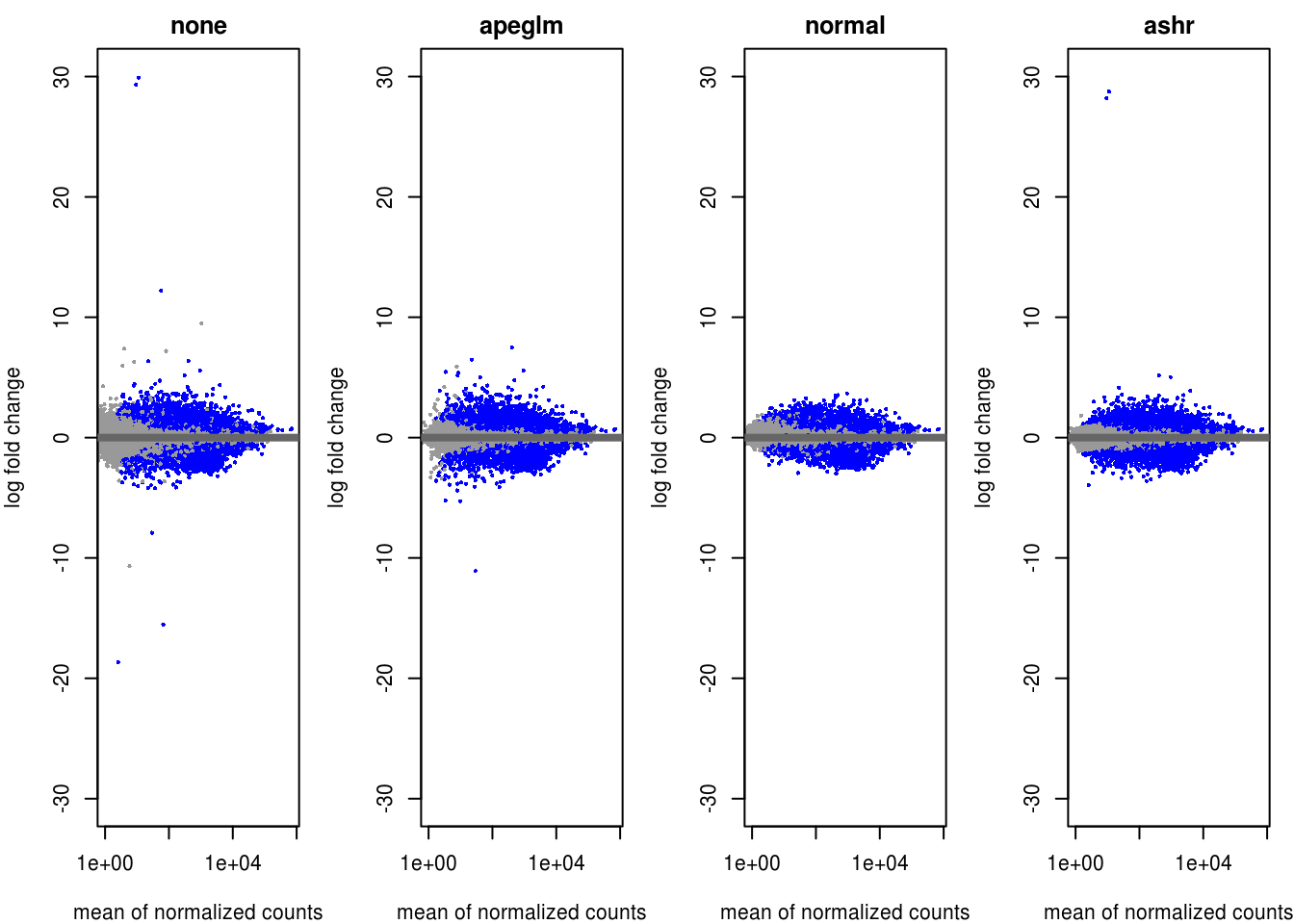

lsf.volcano <- lapply( list(res,resLFC,resNorm,resAsh), function(x){ 
  ggplot(data=data.frame(x) %>% na.omit %>% filter(abs(log2FoldChange) < 15), aes(x=log2FoldChange, y=-log10(padj))) +
        geom_point() + 
        theme_minimal() +
        geom_vline(xintercept=c(-0.6, 0.6), col="red") +
        geom_hline(yintercept=-log10(alpha), col="red") +
        xlim(-15,15) +
        ylim(-5,60)
        })

#do.call("grid.arrange", c(lsf.volcano, ncol=2, nrow=2))

do.call("plot_grid",c(lsf.volcano, labels ="auto"))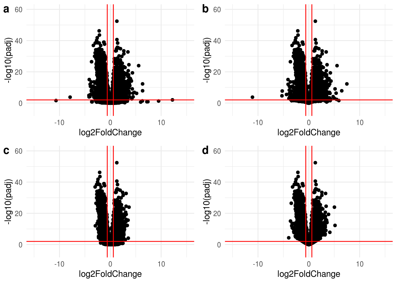

3.3.1.2 DE genes list

 resAsh <-data.frame(resAsh) %>% mutate_if(is.numeric,round,4)
 DT::datatable(resAsh,extensions =c('Buttons'), options = list(
    dom = 'Bfrtip',
    buttons = c('copy', 'csv', 'excel', 'pdf', 'print')
  )) 

3.3.2 Cell lines Comparison

design(dds) <- ~ cell.batch + name

##   Note: levels of factors in the design contain characters other than
##   letters, numbers, '_' and '.'. It is recommended (but not required) to use
##   only letters, numbers, and delimiters '_' or '.', as these are safe characters
##   for column names in R. [This is a message, not a warning or an error]

ddsgrp <- DESeq(dds)

## using pre-existing size factors

## estimating dispersions

## found already estimated dispersions, replacing these

## gene-wise dispersion estimates

## mean-dispersion relationship

##   Note: levels of factors in the design contain characters other than
##   letters, numbers, '_' and '.'. It is recommended (but not required) to use
##   only letters, numbers, and delimiters '_' or '.', as these are safe characters
##   for column names in R. [This is a message, not a warning or an error]

## final dispersion estimates

##   Note: levels of factors in the design contain characters other than
##   letters, numbers, '_' and '.'. It is recommended (but not required) to use
##   only letters, numbers, and delimiters '_' or '.', as these are safe characters
##   for column names in R. [This is a message, not a warning or an error]

## fitting model and testing

## 5 rows did not converge in beta, labelled in mcols(object)$betaConv. Use larger maxit argument with nbinomWaldTest

alpha <- 0.01
threshold <- 1
contrast.group <- ddsgrp@colData %>% as.data.frame  %>% dplyr::select(-c(cell.batch,sizeFactor)) %>% mutate_at("name",as.factor) %>% unique() %>% group_by(cell.line) %>%  group_split(name)
#res.list <- lapply(contrast.group[-c(12)], function(x){ x<- unlist(as.character(x$name)) ; results(ddsgrp,contrast = c("name",x),alpha = alpha)})
res.ashr.list <-  lapply(contrast.group[-c(12)], function(x){ x<- unlist(as.character(x$name)) ; lfcShrink(ddsgrp,contrast = c("name",x), type="ashr")})

yMax <- quantile(sapply(res.ashr.list,function(x){max(abs(x$log2FoldChange),na.rm= TRUE)}),0.75)
yMax <- 10
yMax.padj <- quantile(sapply(res.ashr.list,function(x){max(-log10(x$padj[x$padj >0]),na.rm= TRUE)}),0.85)
xMax <- max(sapply(res.ashr.list,function(x){plotMA(object = x, returnData = T)[,1]}))
xlim <- c(1,xMax); ylim <- c(-yMax, yMax)

volcano.plots <- lapply(res.ashr.list, function(x){plot.volcano(x,ylim,c(-yMax.padj*0.2,yMax.padj),5)})

do.call("plot_grid",c(volcano.plots, labels ="auto",  nrow=6))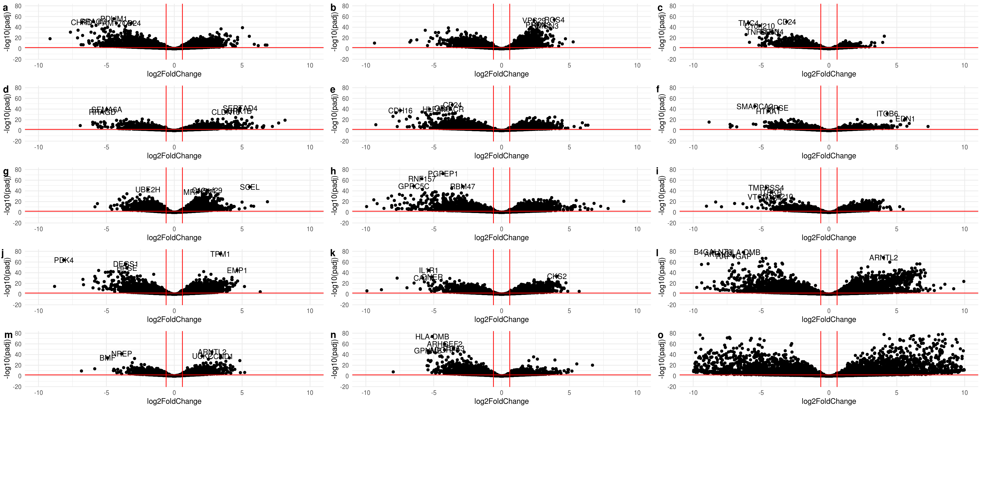

3.3.2.1 DE Gene / Cell Line Summary Table

summary.df <- do.call(cbind,lapply(res.ashr.list,function(x){data.frame(x) %>% dplyr::filter(padj<alpha & abs(log2FoldChange) > threshold) %>% dplyr::select(log2FoldChange) %>% summary %>% str_extract_all("-?[0-9]+.[0-9]+") %>% as.numeric}))
colnames(summary.df) <- ddsgrp@colData %>% as.data.frame  %>% dplyr::select(cell.line) %>% unique %>% slice(-12)  %>% mutate_all(as.character) %>% unname %>% unlist
rownames(summary.df) <- data.frame(res.ashr.list[[1]]) %>% dplyr::filter(padj<alpha & log2FoldChange > threshold ) %>% dplyr::select(log2FoldChange) %>% summary %>% str_extract_all("[1-9][:alpha:]+ [:alpha:]+|[:alpha:]+", simplify =  TRUE)

summary.df <- rbind(summary.df, Count=sapply(res.ashr.list,function(x){data.frame(x) %>% dplyr::filter(padj<alpha & abs(log2FoldChange) > threshold) %>%  dim %>% head(1) %>% as.integer() }) )
kable(summary.df)%>% kable_styling("striped")  %>%scroll_box(width = "100%")

	C5X	ES2	HAC2	HCH1	JHOC5	JHOC9	KOC	OV207	OVAS	OVISE	OVMANA	OVTOKO	SMOV2	TOV21G	RMGII
Min	-9.1504	-10.53484	-17.290	-30.38630	-30.111	-24.6739	-35.3516	-18.0418	-9.0214	-17.0668	-12.6053	-24.5268	-24.2218	-30.9326	-13.519
1st Qu	-2.2497	-1.46009	-1.915	-1.80343	-2.138	-1.5273	-1.3680	-1.9656	-1.7049	-1.7811	-1.7901	-2.4433	-1.3779	-1.7976	-1.919
Median	-1.3674	1.00399	-1.364	-1.00537	-1.252	-1.0920	1.0488	-1.1454	-1.1332	-1.1312	-1.1083	-1.2426	1.1312	-1.1674	1.128
Mean	-0.8333	-0.01715	-1.023	0.02051	-0.666	-0.2558	0.1445	-0.4408	-0.3192	-0.2912	-0.2817	-0.5524	0.3168	-0.4974	0.479
3rd Qu	1.2309	1.49547	1.005	1.91022	1.313	1.4367	1.5807	1.4864	1.4829	1.4818	1.4657	1.5309	1.7226	1.3387	2.799
Max	6.8254	5.27310	12.381	8.15982	6.363	7.2999	6.8632	24.7988	5.4680	14.5713	5.7157	28.9316	41.5569	6.6958	25.399
Count	3532.0000	3170.00000	1519.000	1873.00000	2992.000	2614.0000	3135.0000	3451.0000	1701.0000	3664.0000	2898.0000	5136.0000	1902.0000	2391.0000	6434.000

56 DE genes is found across 16 cell line pairs

DGE.gene.list <- lapply(res.ashr.list,function(x){x %>% as.data.frame %>% dplyr::filter(padj<alpha & abs(log2FoldChange) > threshold)  %>% rownames })
DGE.gene.union.list <- Reduce(union,DGE.gene.list) %>% unique

mtx<- sapply(DGE.gene.list,function(x){tmp<-c();tmp[DGE.gene.union.list %in% x] <- 1 ;return(tmp)})
colnames(mtx) <-  ddsgrp@colData %>% as.data.frame  %>% dplyr::select(cell.line) %>% unique %>% slice(-12)  %>% mutate_all(as.character) %>% unname %>% unlist
rownames(mtx) <- DGE.gene.union.list
mtx[is.na(mtx)] <- 0
upset(data.frame(mtx),nset=15,order.by ="freq" ,point.size = 2, line.size = 1,mainbar.y.label = "DE Genes Overlap #",  sets.x.label = " Total DE Genes")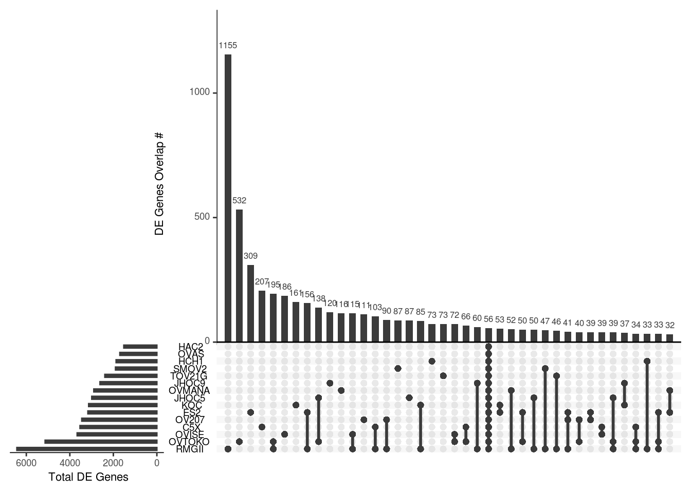

Fold change summary of 56 common DE genes

de.group.select.gene <- rownames(mtx[rowSums(mtx) == max(rowSums(mtx)),])
de.group.df <- do.call( "cbind" ,sapply(res.ashr.list, function(x){x %>% as.data.frame %>%rownames_to_column("gene") %>% dplyr::filter( gene %in% de.group.select.gene) %>% mutate_if(is.numeric,round,4) %>% dplyr::select(log2FoldChange)} ))
colnames(de.group.df) <- colnames(mtx) 
rownames(de.group.df) <- de.group.select.gene
DT::datatable(de.group.df,extensions =c('Buttons', 'Scroller'), options = list(
    dom = 'Bfrtip',
    buttons = c('copy', 'csv', 'excel', 'pdf', 'print'),
    "scrollX"= TRUE
  ))

root.dir <- rprojroot::find_rstudio_root_file()
knitr::opts_chunk$set(echo = TRUE)
knitr::opts_knit$set(root.dir = root.dir )
library(readr)
library(tidyverse)
library(kableExtra)
library(stringr)
library(DiffBind)
source(file.path(root.dir,'src/util.R'))
source(file.path(root.dir,'src/plot_swoosh.R'))